Laser Research
Exploring diverse applications and cutting-edge developments in laser technology
01 Introduction
In precision laser technology, the laser scanning galvanometer is undoubtedly the core execution unit. From millimeter-level industrial marking to micron-level additive manufacturing, galvanometers—with their unparalleled speed and precision—have become a driving force in technological progress.
However, for most engineers engaged in laser application development, galvanometers are both familiar and mysterious.
When laser additive manufacturing faces corner overheating, how can we eliminate it at the control level?
When seamless processing on large workpieces is required, why does the traditional “step-and-scan” mode introduce stitching errors, and how does IFOV (Image Field of View / scan-stage synchronization) technology solve this?
Why are small-aperture galvanometers extremely fast, while large-aperture galvanometers are relatively slow? What physical contradictions lie behind this?
This article will explore the core principles, physics, and control logic of laser scanning galvanometers:
How is the beam movement driven? What irreconcilable conflict exists between motor inertia and optical aperture?
What gap exists between command and execution? Does the system merely passively chase the target (tracking error), or can it actively predict the path (feedforward control)?
How is stability ensured in microsecond-level response? Where do jitter and thermal drift originate?
When the galvanometer collaborates with a motion stage, how are commands intelligently decomposed and scheduled? How can stitching errors be fundamentally eliminated?
scanning galvanometer
02 Scanning Galvanometer Basics: How Does It Work?
To understand a complex system, we must return to its core. This section focuses on the basic physics and concepts of galvanometer technology.
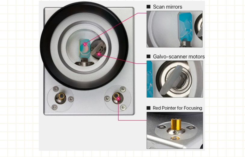
Parts of a scanning galvanometer
1. Everything Begins with Deflection
The essence of laser scanning is precisely controlled deflection of the laser beam. Without deflection, a laser emits only a static beam, with very limited applications. Scanning transforms it into a dynamic tool—able to go wherever commanded—vastly expanding its applications in machining, marking, imaging, and more.
Several deflection technologies exist, each with pros and cons:
Rotating polygon mirror: Extremely fast, but usually limited to periodic 1D scanning (like drum printing).
Acousto-optic/electro-optic deflectors (AOD/EOD): Very fast (nanosecond response), but limited in deflection angle and beam aperture.
Scanning galvanometer: Offers superior speed, precision, and flexible vector addressing. It follows computer commands to quickly and accurately direct the beam to any position on the working plane.
Laser scanner = Galvanometer + EOD/AOD
2. Oscillating Motor
At its core, a galvanometer is a special, high-precision oscillating motor. Its principle is based on Lorentz force:
When a current-carrying coil is placed in a magnetic field, it experiences torque proportional to the current, causing rotation.
Like an ammeter: current deflects the coil, moving the needle.
In galvanometers, the needle is replaced by a mirror. Drive current controls the mirror’s deflection angle.
Through a precise servo control system, the mirror does not rotate continuously but stabilizes at a commanded angle. The driver board converts input voltage signals into accurate drive currents, ensuring precise mirror control.
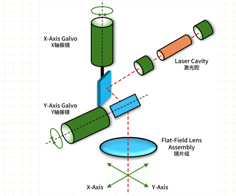
3. Building the Scanning Plane
A typical 2D scanning head has two galvanometers with perpendicular axes:
Laser hits the first mirror (X-axis)
Reflected to the second mirror (Y-axis)
Independent control of both angles directs the laser to any (X,Y) coordinate in the working plane.
This vector-based random addressing is a major advantage over raster-type polygon scanning.
4. Jumping & Marking Modes
Galvanometer movement has two modes, synchronized with laser ON/OFF:
Jump mode (laser OFF): Fast repositioning to the next start point, at maximum speed/acceleration.
Marking mode (laser ON): Controlled speed to meet processing requirements.
Core design contradiction:
Speed demands: Requires strong torque + minimal inertia (small, light mirrors).
Power demands: Requires larger mirrors to handle bigger beams without clipping, especially for high-power lasers.
These are contradictory:
Small-aperture mirrors: Low inertia, very fast → biomedical imaging, small-spot high-dynamics.
Large-aperture mirrors: High inertia, slower → high-power lasers for welding, cutting, 3D printing.
Thus, galvanometer selection is always a trade-off between speed and power capacity.
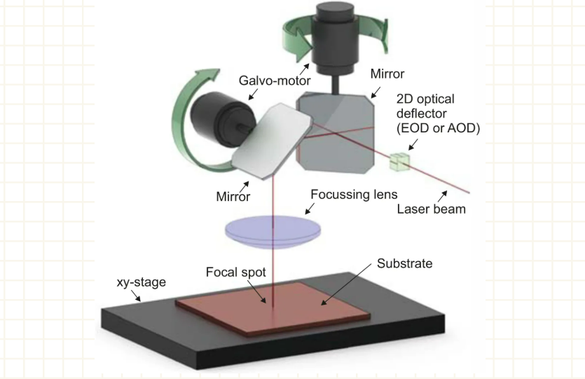
03 A Complete Scanning Galvanometer System
1. System Architecture
Workflow:
Laser source generates beam
Beam collimated and shaped by beam expander
Beam enters scanning head → deflected by X/Y mirrors
Beam passes through F-Theta lens → focused and linearized
Focused spot processes the workpiece
All controlled by software + control card, forming a closed loop from digital command to physical processing.
System diagram
2. Galvanometer Motor
Decides system dynamics. Components:
Stator & rotor
Moving magnet design: Magnet on rotor, coil fixed. Low inertia → higher resonance frequency, faster response. Mainstream.
Moving coil design: Coil on rotor, magnet fixed. Higher torque efficiency but higher inertia → limited speed.
Bearings: Precision preloaded ball bearings ensure rigidity, low friction, and long lifespan.
3. Mirrors
Affect optical quality and power handling.
Aperture: Determines max beam size.
Substrates:
Silicon: Good thermal conductivity, for mid/high-power IR (CO₂, fiber lasers).
Fused silica: Ultra-low thermal expansion, best for UV and ultrafast lasers.
Coatings: High-reflectivity dielectric (>99.5%) at target wavelength.
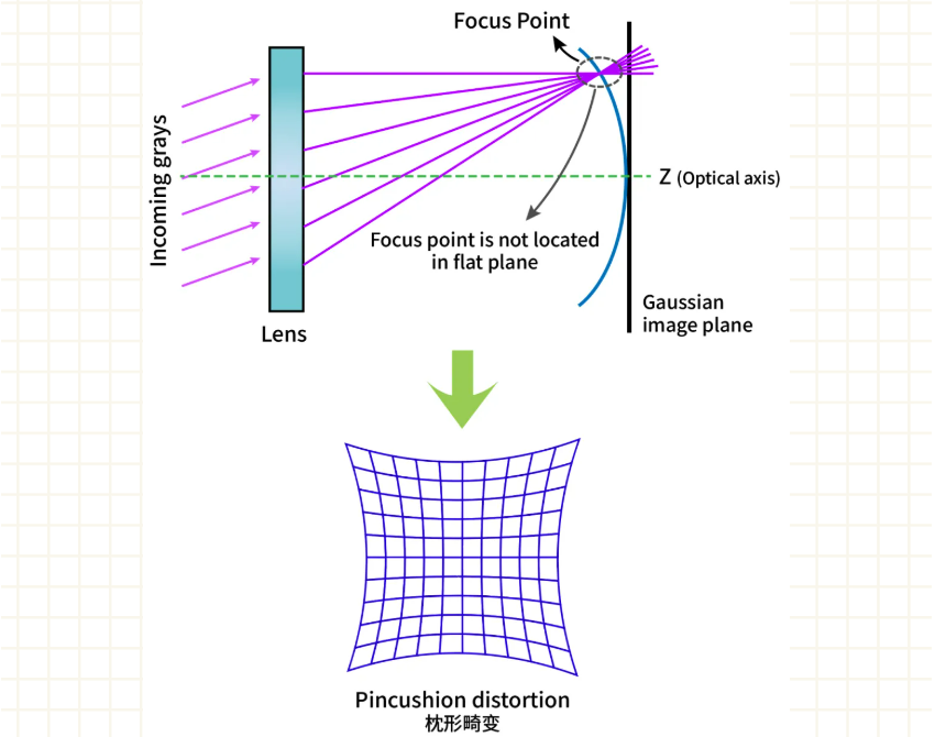
4. F-Theta Lens
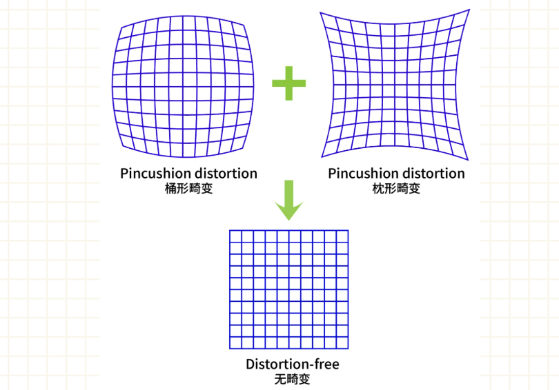
Without it → two fatal issues:
Field curvature: Focused on a curved surface, not flat.
Nonlinearity & distortion: Spot speed varies across field; square becomes pillow-shaped.
Solution: F-Theta lens
Adds barrel distortion to cancel scanning distortion → nearly linear relationship y’≈f·θ.
Functions:
Linear scanning
Flat-field focusing
Uniform spot size & energy density
Without F-Theta Lens
With F-Theta Lens: Introduces Barrel Distortion
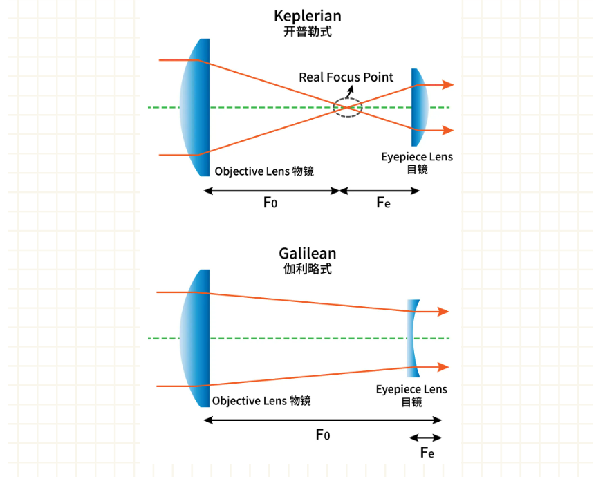
5. Beam Expander
Used before scanning head.
Function: Telescope system enlarges beam diameter.
Effect: Reduces divergence → smaller focused spot, higher resolution.
Types:
Keplerian (two positives, real focus, supports spatial filtering, but risk of air breakdown at high power).
Galilean (negative + positive lens, compact, no internal focus, most common in industry).
Beam Expander: Keplerian & Galilean Types
04 Closed-Loop Servo System
1. Why Closed-Loop?
Open loop: Sends commands but doesn’t check results → drift, load change, interference.
Closed loop: Compares command vs actual (feedback), corrects continuously → precision achieved.
Error = Command – Actual. Controller drives error → 0.
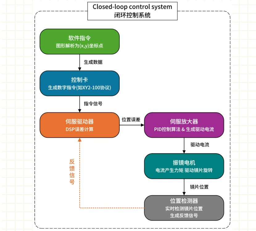
2. From Digital Command to Mirror Deflection
Flow:
Design converted into (X,Y) points
Control card sends signals (e.g., XY2-100) to driver
Driver compares command vs feedback
DSP calculates error → generates drive current via PID or advanced algorithms
Current → torque → mirror moves → feedback updates
Loop repeats thousands of times per second
Closed-Loop Control System of the Galvo Scanner
3. Position Detectors
Types:
Optical (analog): IR LED + shadow mask on rotor → detected by photodiode.
Capacitive (analog): Measures capacitance change with rotation.
Digital encoder (grating): High-resolution disk read optically → digital output, highest precision, lowest drift.
4. Servo Driver
Analog (old): Prone to noise, manual tuning, inflexible.
Digital (modern):
DSP firmware runs control algorithms
Noise immune
Can use predictive feedforward → near-zero tracking error
Key difference:
Analog = reactive, always chasing error
Digital = predictive, plans ahead → solves corner overheating in additive manufacturing.
05 Key Performance Indicators
Speed
Marking speed (mm/s or cps) → efficiency
Jump speed → repositioning time
Step response → stabilization time after deflection
Precision
Accuracy = actual vs commanded
Repeatability = consistency returning to same point
Resolution = smallest deflection step
Stability
Thermal drift = slow position shift due to heating
Jitter = high-frequency oscillations at static position → poor edge quality
06 Control Architecture: Challenges & Solutions
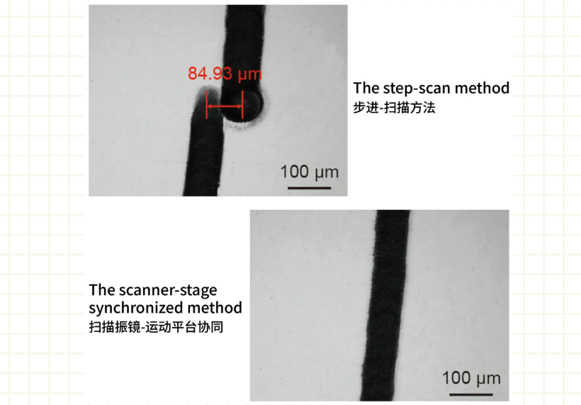
1. Traditional Step-and-Scan
Large stage inertia = slow
Limited FOV = requires stitching (errors appear)
Platform & galvanometer independent = simple sequence execution
Control delays = trajectory distortion
Stitching Error
2. Solution 1: Distortion Correction
Old: Lookup tables (LUT), many measured points, time-consuming
Modern: Sparse data + physical modeling, e.g., only 25 points to model entire field
3. Solution 2: Infinite Field of View (IFOV)
Also called galvo-stage synchronization
Unified controller coordinates both systems
Path decomposition:
Low-frequency, long moves → stage
High-frequency, fine details → galvo
Error correction:
Predictive planning or real-time compensation
4. Solution 3: Precision Synchronization
Direct drive (PWM): Controller bypasses drivers, talks directly to motor → reduces delay
Position-Synchronized Output (PSO): Laser pulses triggered by distance, not time → consistent energy density, solves corner overheating
Advanced power control: Real-time power adjustment ensures constant energy density
Goal: Stable process parameters → predictable physical results
07 Conclusion
The scanning galvanometer is no longer a simple 2D beam deflector.
Past: Independent actuator (motor + mirror), following input signals.
Now: Integrated subsystem with Z-axis focusing, built-in digital controllers, diagnostic data streaming.
Future: Possible deep integration with robots, motion stages, real-time data exchange → true smart manufacturing.
Contact us to get the latest galvanometer solutions
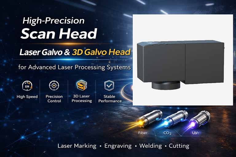
Scan Head & 3D Galvo Head for Laser Systems
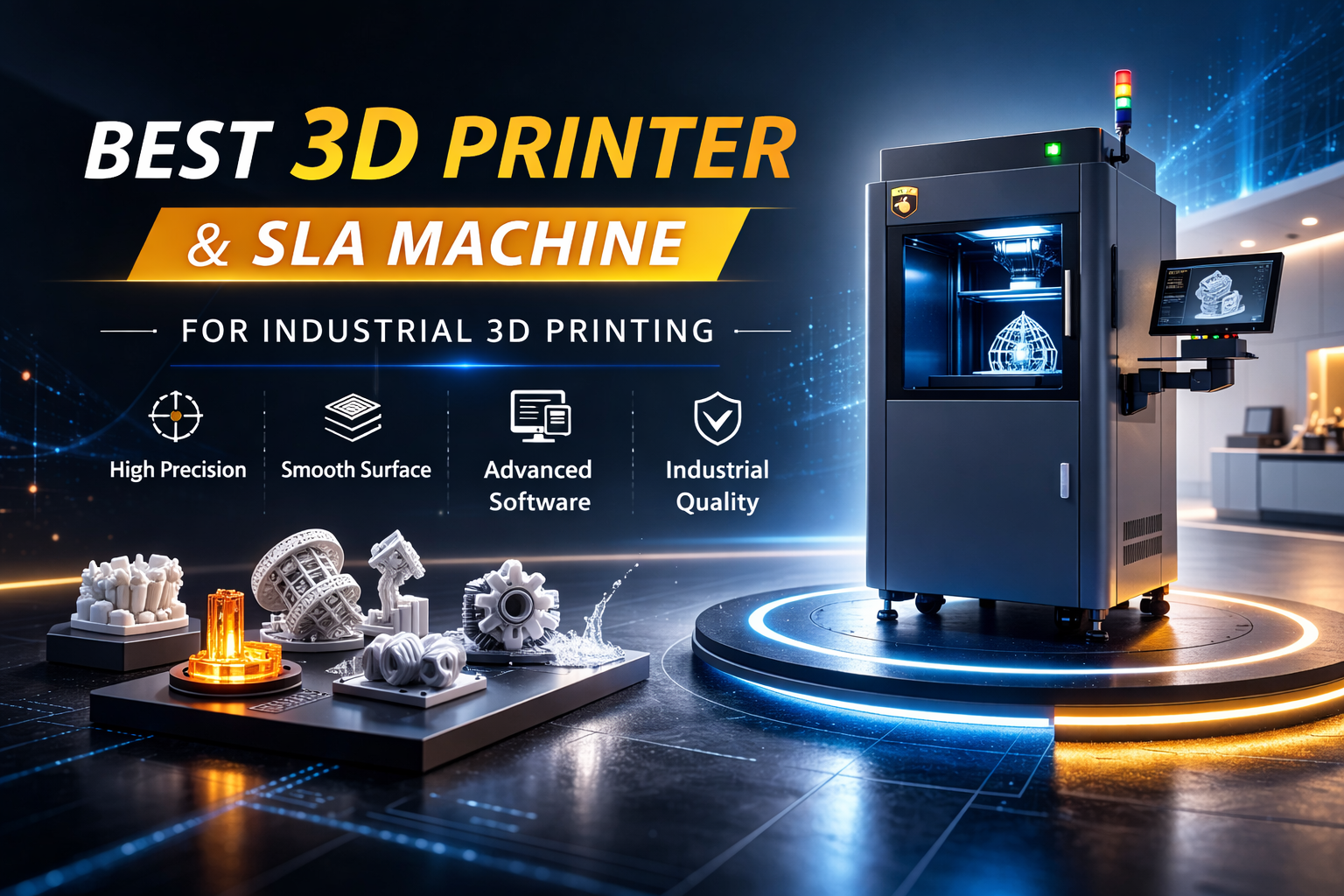
Best 3D Printer & SLA Machine for Industrial 3D Printing
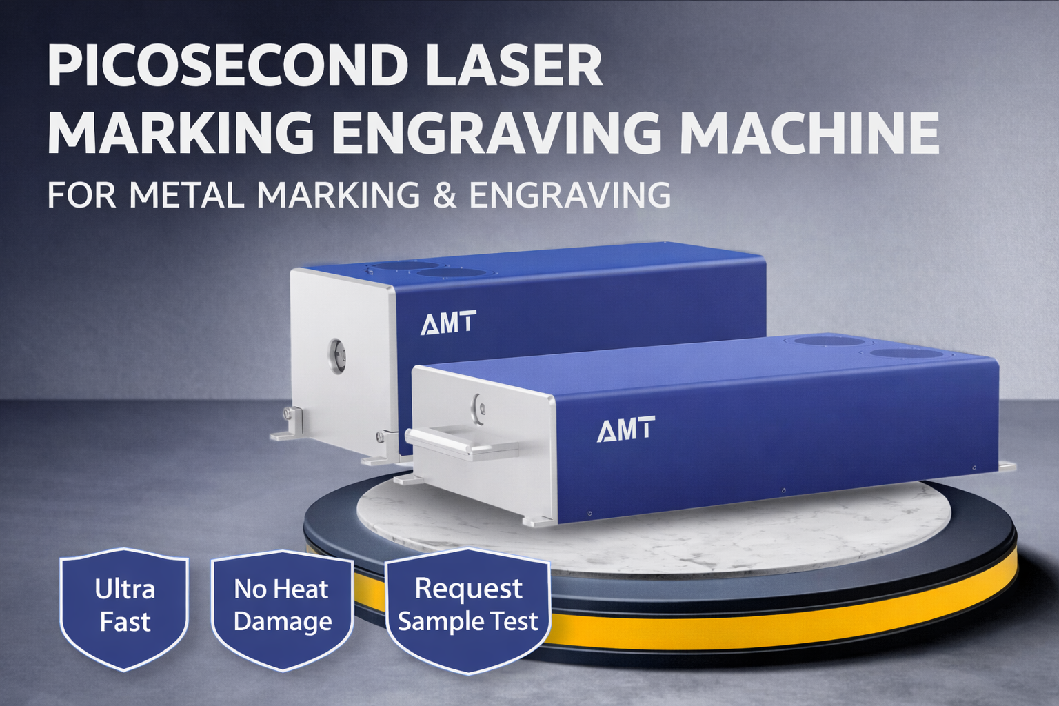
Picosecond Lasers for Ultra-Precision Metal Marking & Engraving
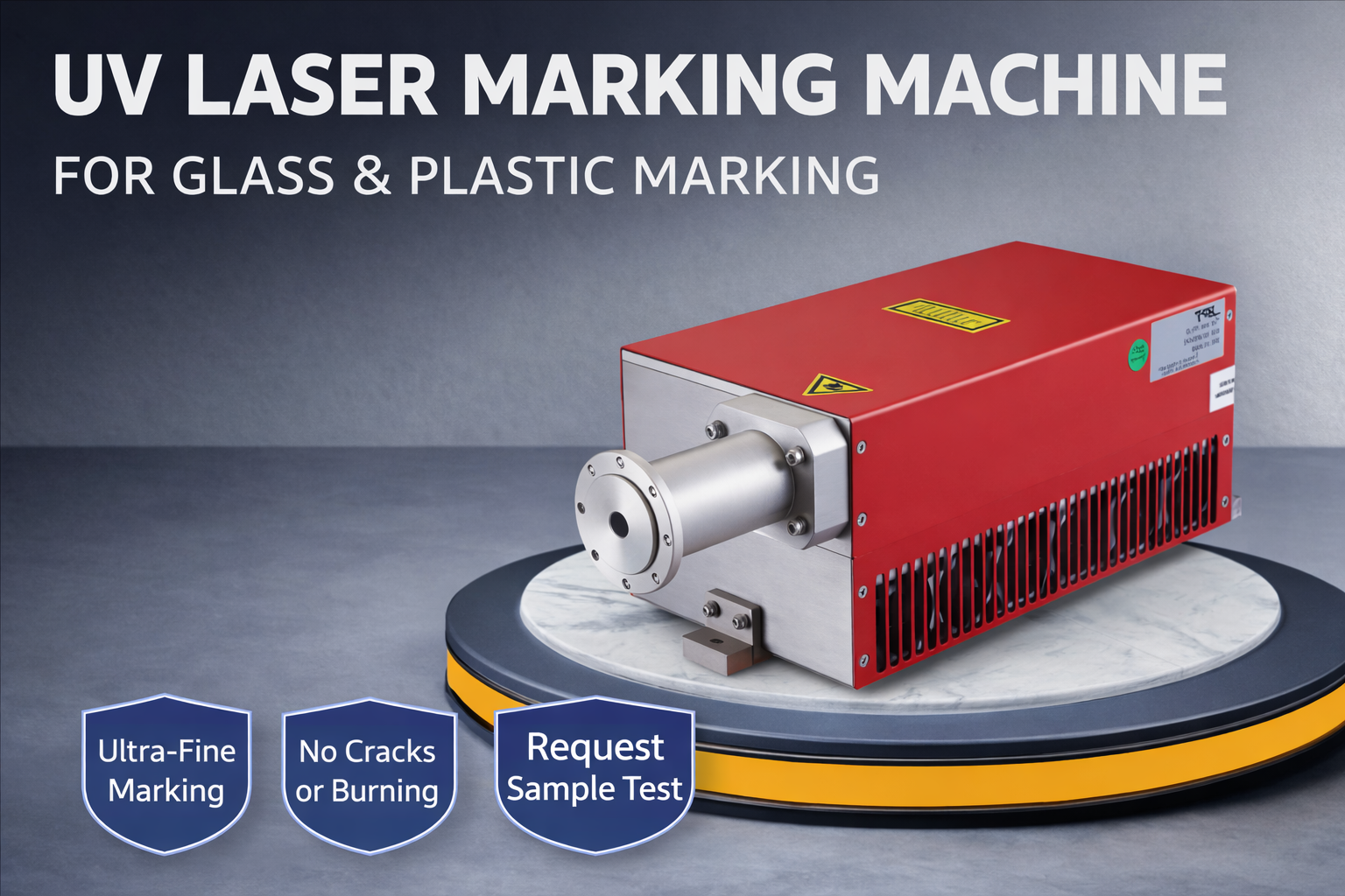
UV Laser Marking Machine for Glass, Plastic & High-Precision Applications
High Performance Nanosecond Lasers for Industrial Precision Processing